character table of \(S_5\)

Let’s use GAP to find the character table of \(S_5\).

gap> G:=SymmetricGroup(5);
Sym( [ 1 .. 5 ] )
gap> tab:=CharacterTable(G);
CharacterTable( Sym( [ 1 .. 5 ] ) )
gap> Display(tab);
CT1

     2  3  2  3  1  1  2  .
     3  1  1  .  1  1  .  .
     5  1  .  .  .  .  .  1

       1a 2a 2b 3a 6a 4a 5a
    2P 1a 1a 1a 3a 3a 2b 5a
    3P 1a 2a 2b 1a 2a 4a 5a
    5P 1a 2a 2b 3a 6a 4a 1a

X.1     1 -1  1  1 -1 -1  1
X.2     4 -2  .  1  1  . -1
X.3     5 -1  1 -1 -1  1  .
X.4     6  . -2  .  .  .  1
X.5     5  1  1 -1  1 -1  .
X.6     4  2  .  1 -1  . -1
X.7     1  1  1  1  1  1  1
gap> 

Diaconis example – survey data

This data is taken from the paper (Diaconis 1989)

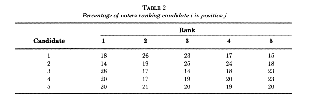
It describes 5,738 completed ballots rank-ordering 5 candidates.

View a rank-ordered ballot as an element of the symmetric group \(S_5\); we want to study the frequency function \(f\).

first ranking table

the regular representation

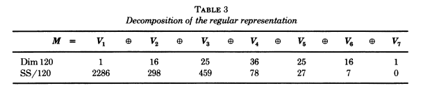
This diagram shows the decomposition of the regular representation into isotypic components.

Be careful: the notation Diaconis is using here does not match that used by GAP above. For example, the representation Diaconis writes as \(V_3\) is the isotypic component determined by the irreducible representation labeled X.5 by GAP.

The second row reflects the decomposition of the frequency function \(f\). Namely, write \[f = \sum_{i=1}^7 f_i \quad \text{with $f_i \in V_i$}.\]

The second row entries are the “sums of squares” \(\langle f_i,f_i \rangle\).

Remember that we can compute the \(f_i\) using the idempotents in \(\mathbb{C}[G]\).

For example,

\[f_1 = \dfrac{1}{5!} \sum_{\sigma \in S_5} \sigma.f\]

More generally, if \(\chi_i\) denotes the character of the irreducible representation \(L_i\) with \(V_i = \mathbb{C}[G]_{(L_i)}\) then \[f_i = \dfrac{1}{5!} \sum_{\sigma \in S_5} \chi_i(\sigma^{-1}) \sigma.f\]

Note that \(\langle f_3,f_3 \rangle = 459\) is relatively large (ignoring \(\langle f_1,f_1 \rangle\) since \(f_1\) is trivial).

normalizing the first-order data

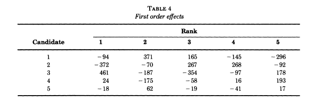
THe \(i,j\) entry in this table is the number of votes ranking candidate \(i\) in the \(j\)-th position, minus the sample size over 5.

In particular, rows and columns sum to 0.

This normalization can also be achieved as follows:

Let \(f_2\) be the projection on \(V_2\), and consider the functions \[\sigma \mapsto \delta_{i,\sigma(j)}.\]

The \(i,j\) entry of the preceding table is \(\langle f_2 , \delta_{i,\sigma(j)} \rangle\)

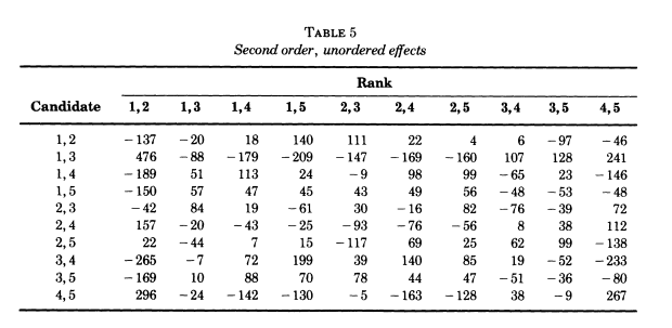
Interpretation in this last table:

Compute the projection \(f_3\) of \(f\) into the component \(V_3\) of \(M = \mathbb{C}[S_5]\).

Now, consider the easily understood functions \[\sigma \mapsto \delta_{\{i,i'\},\{\sigma(j),\sigma(j')\}}\] in \(\mathbb{C}[S_5]\) for distinct \(i,i'\) and distinct \(j,j'\).

The space of these functions is a 100 dimensional subspace of \(W\) \(\mathbb{C}[G]\).

The entries in the table are the inner products \[\langle f_3 , \delta_{\{i,i'\},\{\sigma(j),\sigma(j')\}} \rangle\]

Summary observations

The data were to elect a president for the American Psychological Association. Candidates 1 and 3 were clinicians while candidates 4 and 5 were academicians, two groups within the association with somewhat divergent perspectives.

In the second-order table, we see a preference for candidates 1 & 3 witnessed by the entry 376 corresponding to the entry for candidates \(\{1,3\}\) and ranks \(\{1,2\}\).

And we see a (slightly smaller) preference for candidates 4 and 5 witnessed by the entry 296 corresponding to the entry for candidates \(\{4,5\}\) and ranks \(\{1,2\}\).

Bibliography